1.1.2 Hist

Hist is a Octave class which represents a multi-dimensional histogram. It is useful for accumulating data of a statistical nature and determining its properties.

A one-dimensional histogram is created with the following command:

octave> hgrm = Hist(1, {"lin", "dbin", 0.01})
hgrm = {histogram: count=0, range=[NaN,NaN]}

This histogram will store data in bins with linear boundaries of width 0.01. The Hist class can also store data in bins with logarithmic boundaries:

octave> Hist(1, {"log", "minrange", 0.02, "binsper10", 20})
ans = {histogram: count=0, range=[NaN,NaN]}

To add data to a histogram, use the addDataToHist() function. Let’s add some Gaussian-distributed data:

octave> hgrm = addDataToHist(hgrm, normrnd(10.7, 3.42, [1e4, 1]))
hgrm = {histogram: count=10000, range=[-1.44,22.8]}

We can call addDataToHist() many time to add more data to the histogram:

octave> hgrm = addDataToHist(hgrm, normrnd(10.7, 3.42, [1e4, 1]))
hgrm = {histogram: count=20000, range=[-1.86,24.05]}
octave> hgrm = addDataToHist(hgrm, normrnd(10.7, 3.42, [1e4, 1]))
hgrm = {histogram: count=30000, range=[-2.05,24.05]}
octave> hgrm = addDataToHist(hgrm, normrnd(10.7, 3.42, [1e4, 1]))
hgrm = {histogram: count=40000, range=[-2.42,24.05]}
octave> hgrm = addDataToHist(hgrm, normrnd(10.7, 3.42, [1e4, 1]))
hgrm = {histogram: count=50000, range=[-2.42,24.05]}

We can now compute some basic statistical properties of the data, e.g.:

• mean:

  octave> meanOfHist(hgrm)
  ans =  10.730
  

• standard deviation:

  octave> stdvOfHist(hgrm)
  ans =  3.3879
  

• cumulative distribution:

  octave> arrayfun(@(x) cumulativeDistOfHist(hgrm, x), meanOfHist(hgrm) + (-2:2)*stdvOfHist(hgrm))
  ans =
  
     0.023173   0.157702   0.501401   0.841628   0.977569
  
  

• quantile function:

  octave> arrayfun(@(p) quantileFuncOfHist(hgrm, p), 0.5 + 0.5*[-0.95, -0.68, 0, 0.68, 0.95])
  ans =
  
      4.0630    7.3755   10.7183   14.0960   17.3700
  
  octave> (ans - meanOfHist(hgrm)) / stdvOfHist(hgrm)
  ans =
  
    -1.9679992  -0.9902454  -0.0035522   0.9934369   1.9598407
  
  

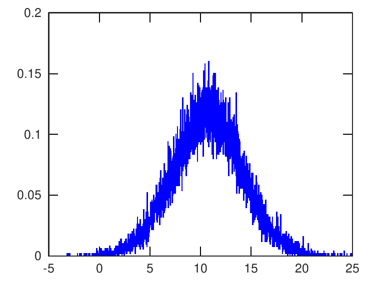
The histogram can also be plotted:

octave> graphics_toolkit gnuplot
octave> plotHist(hgrm, "b");
ezprint("Hist-plot-1.png", "width", 180, "fontsize", 6);

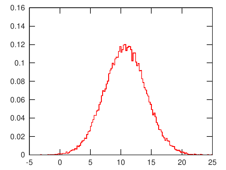
The bin size can be changed by resampling the histogram to a coarser bin size:

octave> plotHist(resampleHist(hgrm, -5:0.2:25), "r");
octave> ezprint("Hist-plot-2.png", "width", 180, "fontsize", 6);

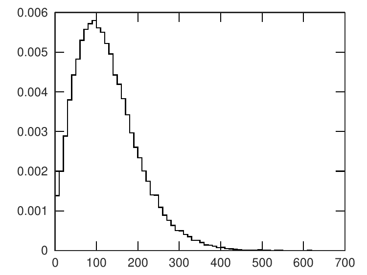
Histograms can be transformed by an arbitrary function. Here we plot the histogram of the squares of the samples:

octave> plotHist(resampleHist(transformHist(hgrm, @(x) x.^2), -10:10:650), "k");
octave> ezprint("Hist-plot-3.png", "width", 180, "fontsize", 6);

Further histogram functions are documented in the histograms and histograms/@Hist directories.