Next: LatticeMismatchHist(), Previous: DoFstatInjections(), Up: Continuous-Wave Functions [Contents][Index]
ComputeDopplerMetric()ComputeDopplerMetric() computes the parameter-space metric which determines the template resolution of continuous gravitational-wave searches.
We compute the metric in the frequency and spindown parameters:
octave> Alpha = 3.92;
octave> Delta = 0.83;
octave> Freq = 200;
octave> f1dot = 1e-9;
octave> Tobs = 86400;
octave> metric = ComputeDopplerMetric("coords", "freq,fdots", "spindowns", 1, "segment_list", 850468953 + [0,Tobs], "ref_time", 731163327, "fiducial_freq", Freq, "detectors", "H1,L1", "det_motion", "spin+orbit", "alpha", Alpha, "delta", Delta);
octave> metric.g_ij
ans =

   2.4559e+10   2.9311e+18
   2.9311e+18   3.4982e+26
We can use the metric to generate random frequency and spindown offsets with random metric mismatches:
octave> dx = randPointInNSphere(2, 0.1 * rand(1, 500));
octave> dfndot = inv(chol(metric.g_ij)) * dx;
octave> mu = dot(dfndot, metric.g_ij * dfndot);
octave> [min(mu), max(mu)]
ans =

   1.9605e-04   9.9810e-02
We can use the generated offsets to compute the F-statistic with DoFstatInjections() to compute the actual mismatch:
octave> DFIargs = {"ref_time", 731163327, "start_time", 850468953, "time_span", Tobs, "detectors", "H1,L1", "sft_time_span", 1800, "sft_overlap", 0, "sft_noise_window", 50, "inj_h0", 0.55, "inj_cosi", 0.31, "inj_psi", 0.22, "inj_phi0", 1.82, "inj_alpha", Alpha, "inj_delta", Delta, "inj_fndot", [Freq; f1dot], "Dterms", 8, "randSeed", 1234};
octave> sch_fndot = [Freq + dfndot(1,:); f1dot + dfndot(2,:)];
octave> sch_Alpha = Alpha * ones(size(sch_fndot(1,:)));
octave> sch_Delta = Delta * ones(size(sch_fndot(1,:)));
octave> res = DoFstatInjections(DFIargs{:}, "det_sqrt_PSD", 1.0, "OrbitParams", false, "sch_fndot", sch_fndot, "sch_alpha", sch_Alpha, "sch_delta", sch_Delta);
octave> res0 = DoFstatInjections(DFIargs{:}, "det_sqrt_PSD", 1.0, "OrbitParams", false);
octave> sch_mu = (res0.sch_twoF - res.sch_twoF') ./ res0.sch_twoF;
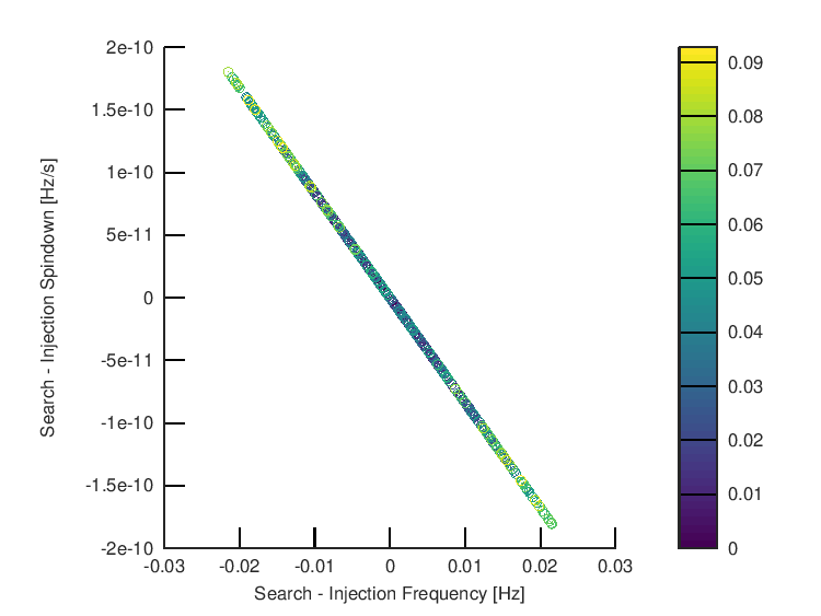
We can plot the actual F-statistic mismatches as a function of frequency and spindown offsets:
octave> graphics_toolkit gnuplot;
octave> scatter(sch_fndot(1,:) - Freq, sch_fndot(2,:) - f1dot, [], sch_mu);
octave> colorbar;
octave> xlabel("Search - Injection Frequency [Hz]");
octave> ylabel("Search - Injection Spindown [Hz/s]");
octave> set(gca, "position", [0.2, 0.11, 0.55, 0.815]);
octave> ezprint("ComputeDopplerMetric-plot-1.png", "width", 180, "fontsize", 4);
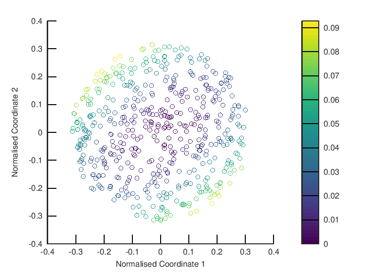
Due to significant correlations between parameters, it is often better to plot in the normalised coordinates dx:
octave> scatter(dx(1,:), dx(2,:), [], sch_mu);
octave> colorbar;
octave> xlabel("Normalised Coordinate 1");
octave> ylabel("Normalised Coordinate 2");
octave> ezprint("ComputeDopplerMetric-plot-2.png", "width", 180, "fontsize", 4);
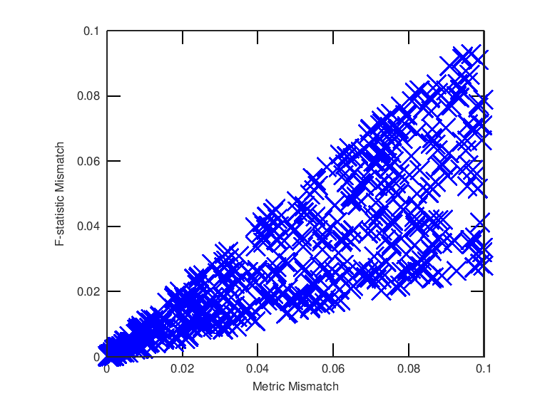
Finally, we can compare F-statistic and metric mismatches:
octave> plot(mu, sch_mu, "bx");
octave> xlabel("Metric Mismatch");
octave> ylabel("F-statistic Mismatch");
octave> set(gca, "position", [0.2, 0.11, 0.705, 0.815]);
octave> ezprint("ComputeDopplerMetric-plot-3.png", "width", 180, "fontsize", 4);
Next: LatticeMismatchHist(), Previous: DoFstatInjections(), Up: Continuous-Wave Functions [Contents][Index]